01 · The measurement bottleneck
Enteric methane is large, and hard to measure at scale
Enteric methane from cattle is one of agriculture's largest greenhouse-gas sources: globally, cattle rival the passenger-car fleet in climate warming. Feed additives, diet changes, and selective breeding can all lower emissions, but proving those reductions requires measuring many animals—and measurement remains the bottleneck.
More than 95% of a cow's enteric methane exits through the nose and mouth via eructation (belching) and exhaled breath. Standard methods rely on sealed respiration chambers or SF₆ tracer halters. Whereas each eructation lasts only seconds, existing instruments report averages over minutes to days.
| Technique | Hardware cost | Invasiveness | Setting | Time resolution |
|---|---|---|---|---|
| Respiration chamber | Up to $2M (facility) | Confinement | Sealed room | τ ≈ 8–10 min (chamber turnover) |
| GreenFeed (C-Lock) | Moderate | Voluntary feeder visits | Barn or pasture | 3–7 min per visit |
| SF₆ tracer gas | Moderate | Rumen bolus and halter | Barn or pasture | Hours to days |
| Mid-infrared optical gas imaging (this work) | < $0.1M (camera) | Non-invasive | Chamber and barn | 30 frames/s (single breaths) |
The gap: no existing method is simultaneously non-invasive, scalable, cost-effective, and operable in the animal's natural environment. Optical gas imaging developed for the oil and gas industry can be repurposed for our application.
References: IPCC AR5 WG1 Ch. 8 (2014); Bannink et al. (2011); Tseten et al. (2022); Hammond et al., Anim. Prod. Sci. 56:181 (2016), GreenFeed; Pinares-Patiño et al., GRA Technical Manual on Respiration Chamber Designs (2014). Hardware costs are indicative.
02 · Mid-infrared radiative transfer
Methane absorbs and emits at 3.3 µm
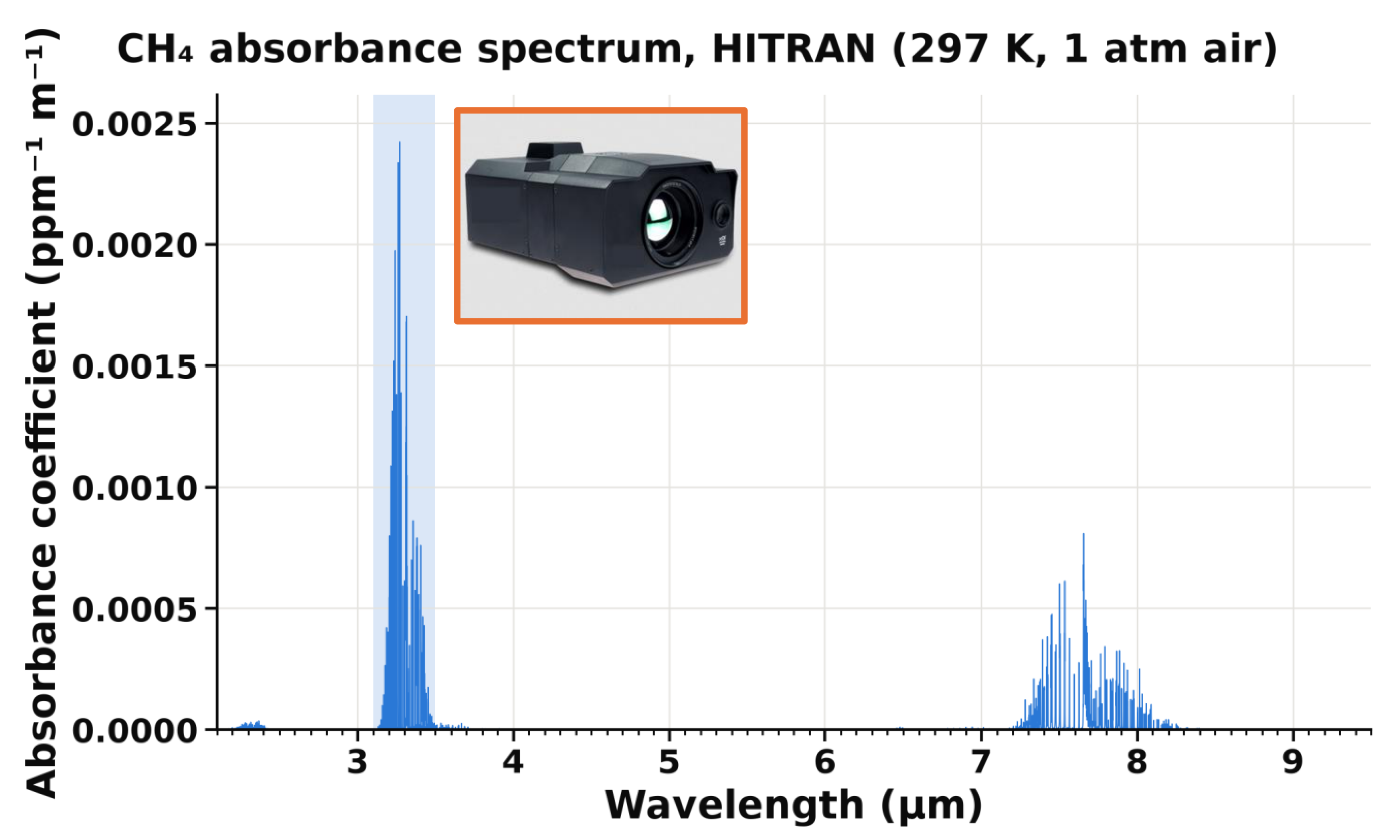
Methane strongly absorbs and emits infrared radiation around 3.3 µm. Our cooled FLIR GIS-320 camera (GF320 core) restricts sensitivity to 3.2–3.4 µm, so a methane plume registers as a radiance change against the background.
A plume produces contrast only when its temperature differs from the background: warm breath in front of a cooler wall adds radiance, whereas gas at the wall's temperature is invisible. We therefore line each chamber with a matte black backdrop (Krylon flat black paint, mid-infrared emissivity ≈ 0.95 or higher), suppressing thermal reflections of the warm cow so the camera views a uniform background temperature.
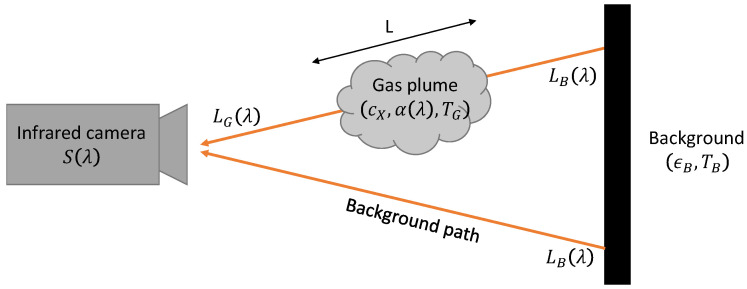
The sensor measures background radiation transmitted through the plume plus radiation emitted by the gas itself. Subtracting the unobstructed background gives the radiance contrast:
Here \(c_X L\) is the methane column density (concentration × path length), \(\alpha\) is the absorption coefficient, and \(L_0(T)\) is the blackbody radiance at temperature \(T\). Either zero methane or zero temperature contrast yields zero signal.
03 · Field proof of concept
First trials in a working dairy barn
Before deploying in respiration chambers, we tested a battery-powered portable OGI rig at Fairvue Farms, a family-owned dairy in Woodstock, Connecticut, to verify that the camera could resolve cow breath plumes along an active feed bunk.
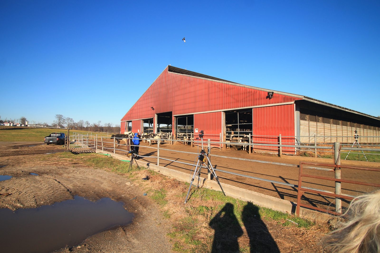
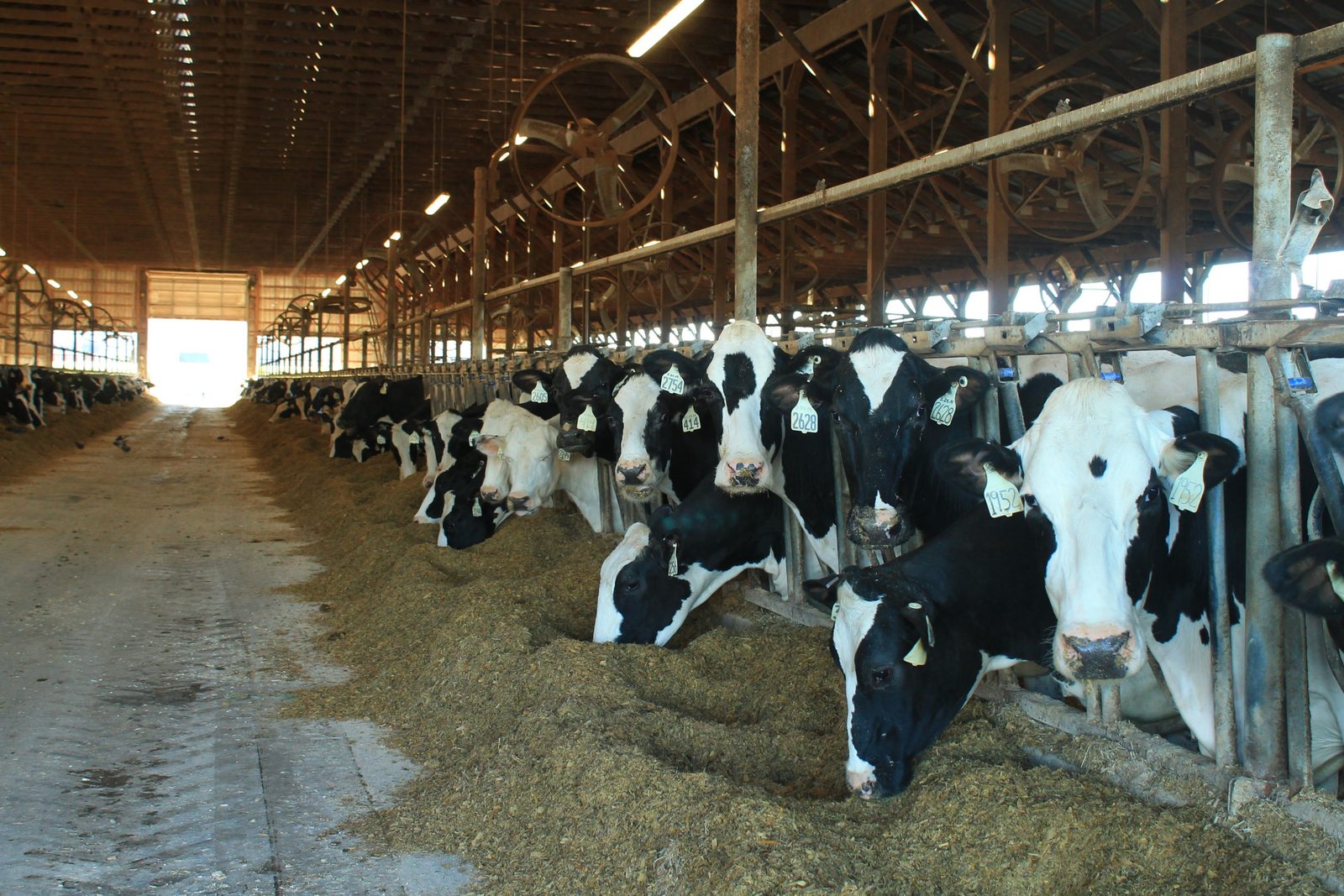
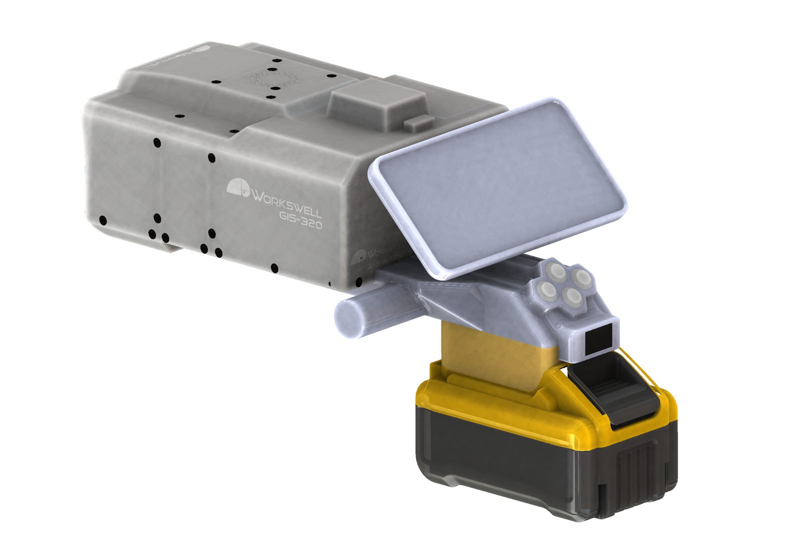
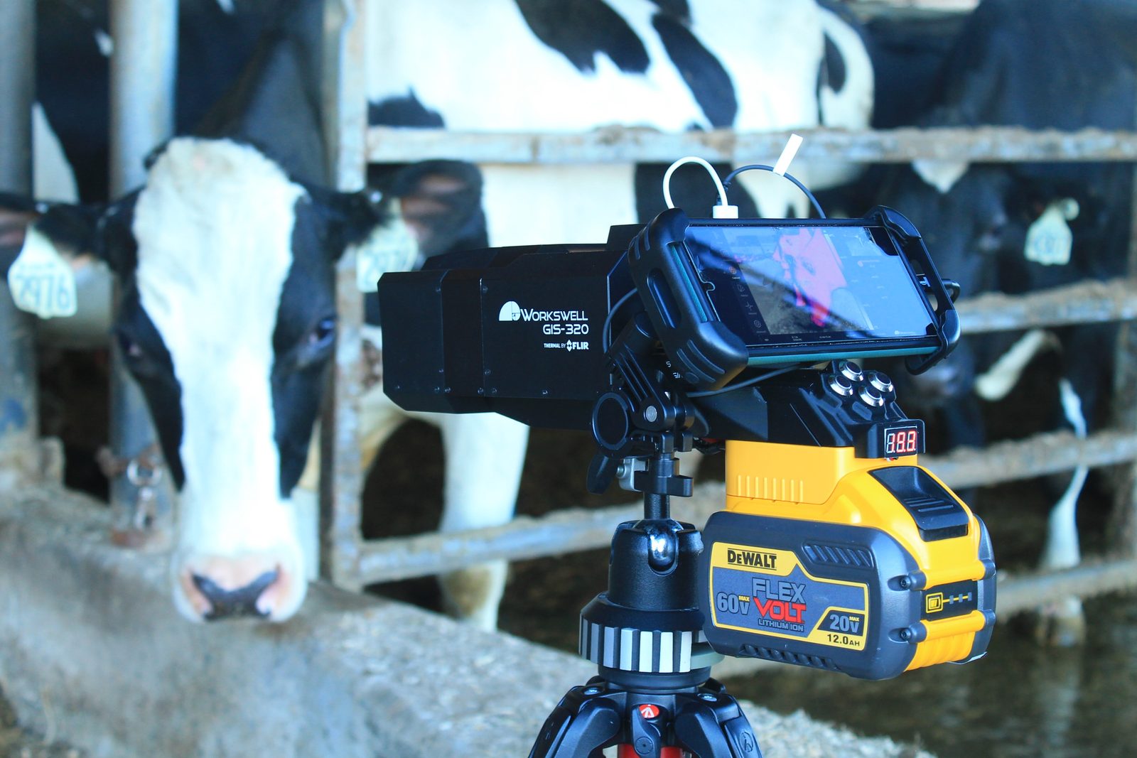
Visualising an eructation at the feed bunk
The barn trial showed that OGI resolves breath plumes alongside natural behaviour, but could not tell us how much methane each plume carries. Quantifying emissions required co-locating the camera with a simultaneous reference instrument: a respiration chamber.
04 · Chamber integration & autonomous tracking
Co-locating the camera with reference gas analysers
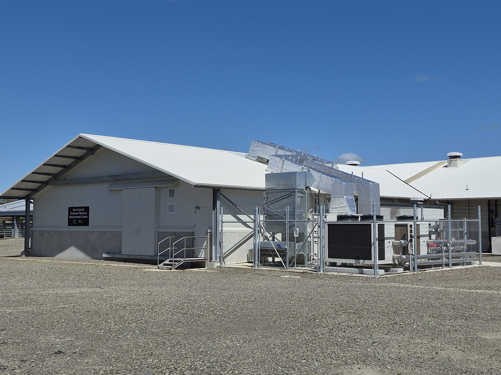
A respiration chamber is a sealed stall ventilated at a known airflow rate while gas analysers measure methane in the exhaust stream. We installed our OGI payload inside chambers at Cornell University and at the New Zealand Ruminant Methane Measurement Centre in Palmerston North (Bioeconomy Science Institute, formerly AgResearch) so the camera and chamber monitor the same cow simultaneously.
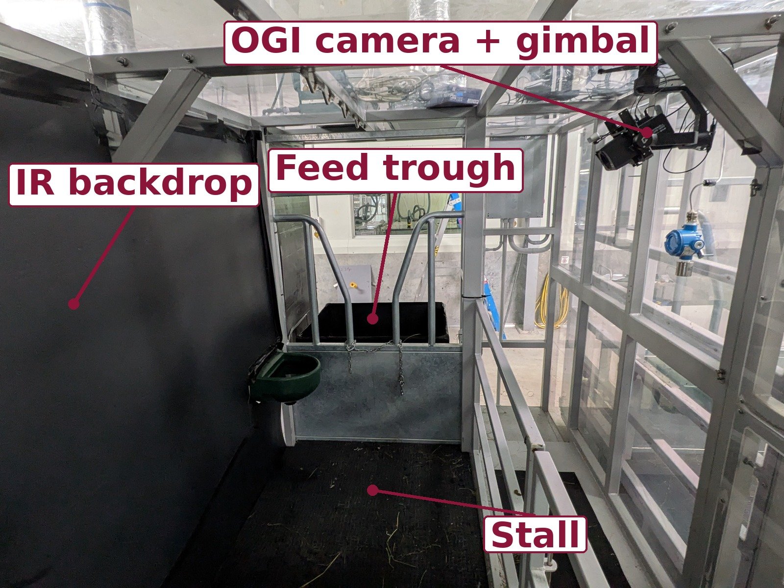
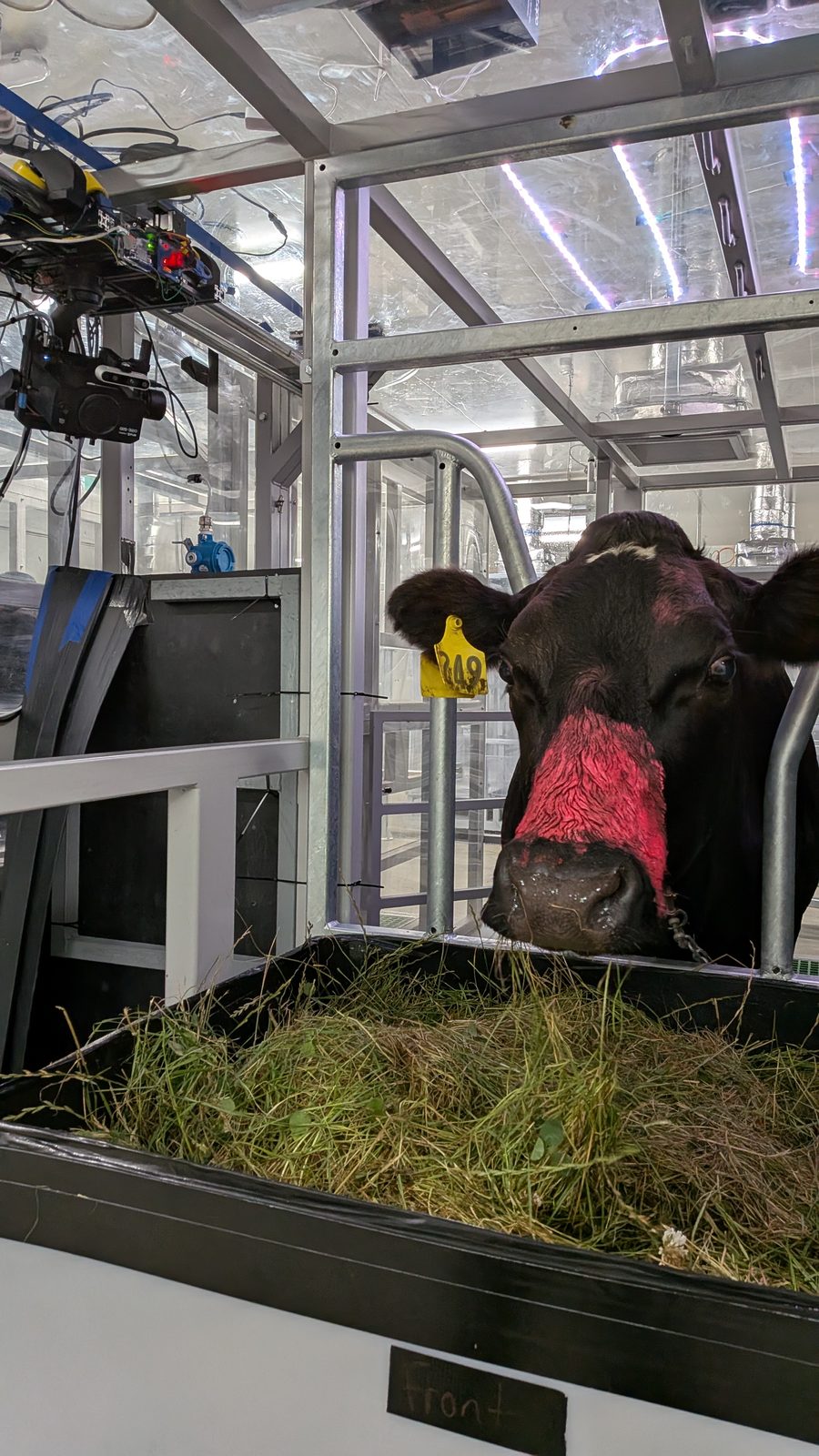
With a cow in the stall. Seen from the front, the cow eats from the feed trough with its nose just through the headgate, while the OGI camera on its gimbal hangs from the chamber frame above. From the camera's side, the head is framed against the black backdrop.
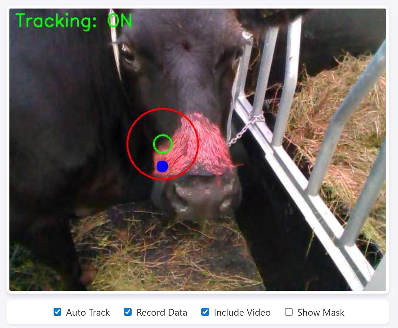
The pink stripe of tail paint on the nose bridge is the marker the tracker follows to keep the nostrils in view (see the ceiling rail and nose tracking below).
Cornell University
Photos and videos from the Cornell chambers are pending permission.
First-generation camera payload, mounted on the chamber wall:
- FLIR GIS-320 cooled OGI camera (mid-IR methane and visible channels)
- Intel RealSense camera (depth and colour video)
- Gremsy T7 two-axis gimbal for remote pointing
- Jetson computer with a 5 TB drive for recording, streaming, and networking
- HDMI transmitter for local wireless viewing, plus a Digilent board and RC receiver for gimbal commands
Because the cow alternates between lying down and standing at the trough, the black backdrop must span both viewing angles.
New Zealand Ruminant Methane Measurement Centre, Bioeconomy Science Institute
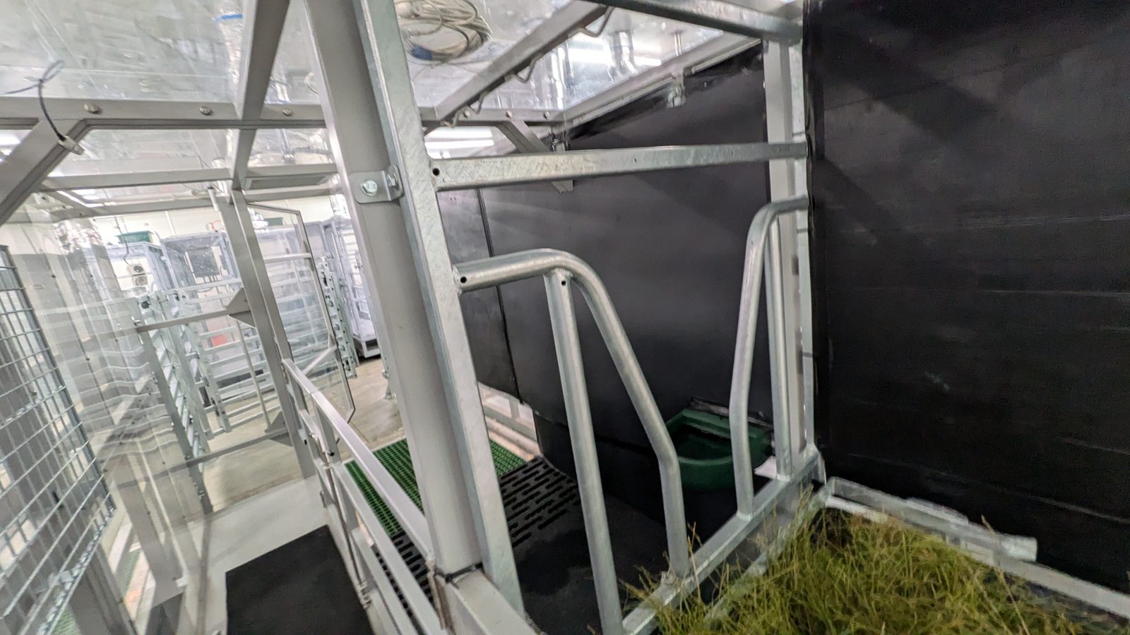
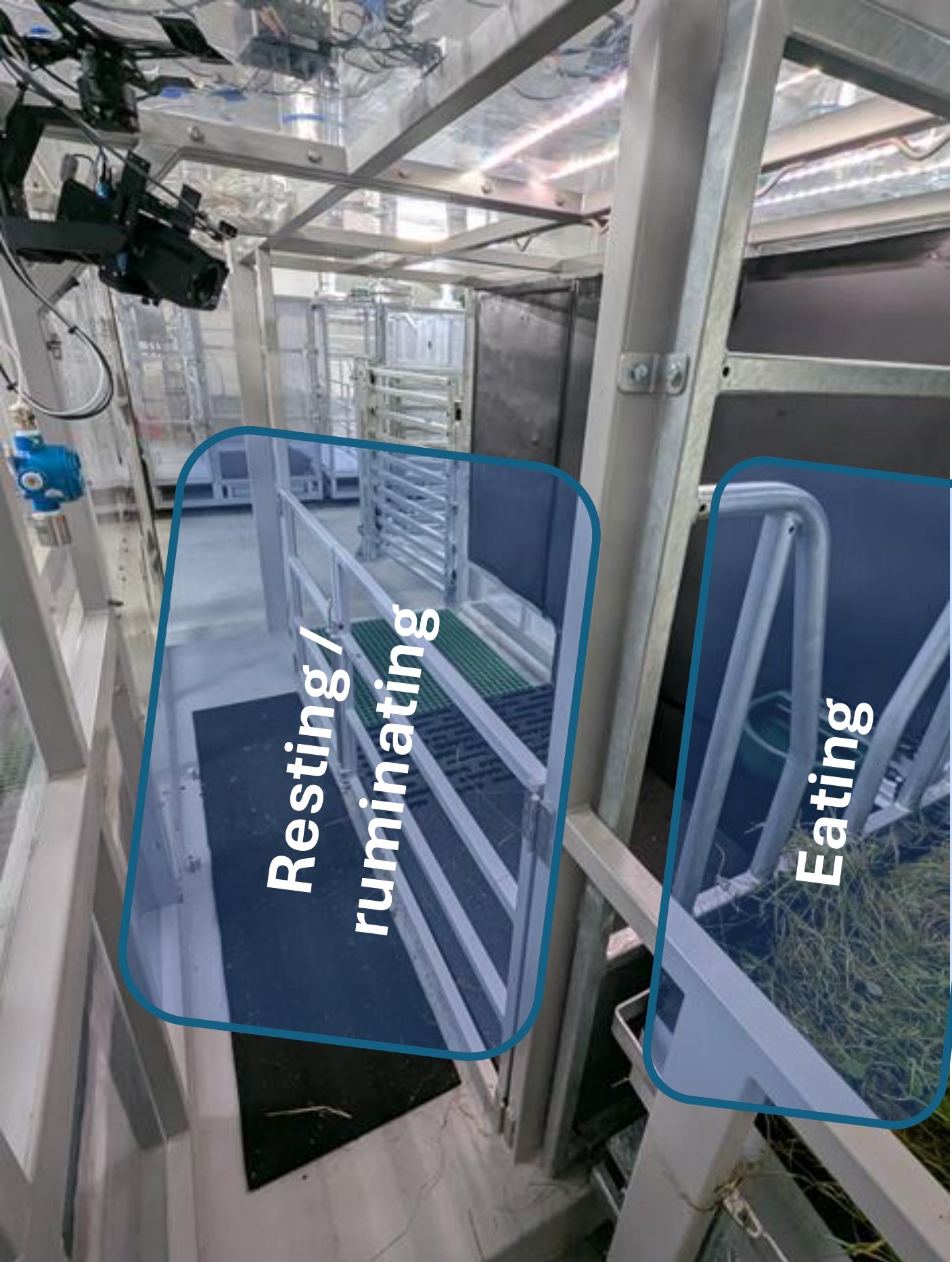
Here the camera payload hangs from the overhead chamber frame looking down on both zones. To follow the cow between resting and feeding positions, we subsequently mounted the payload on a motorized ceiling rail.
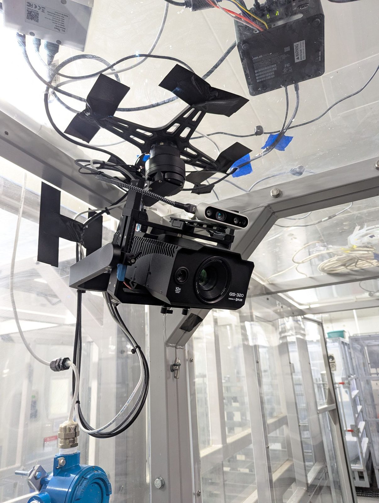
Motorized ceiling rail and 15 Hz nose tracking
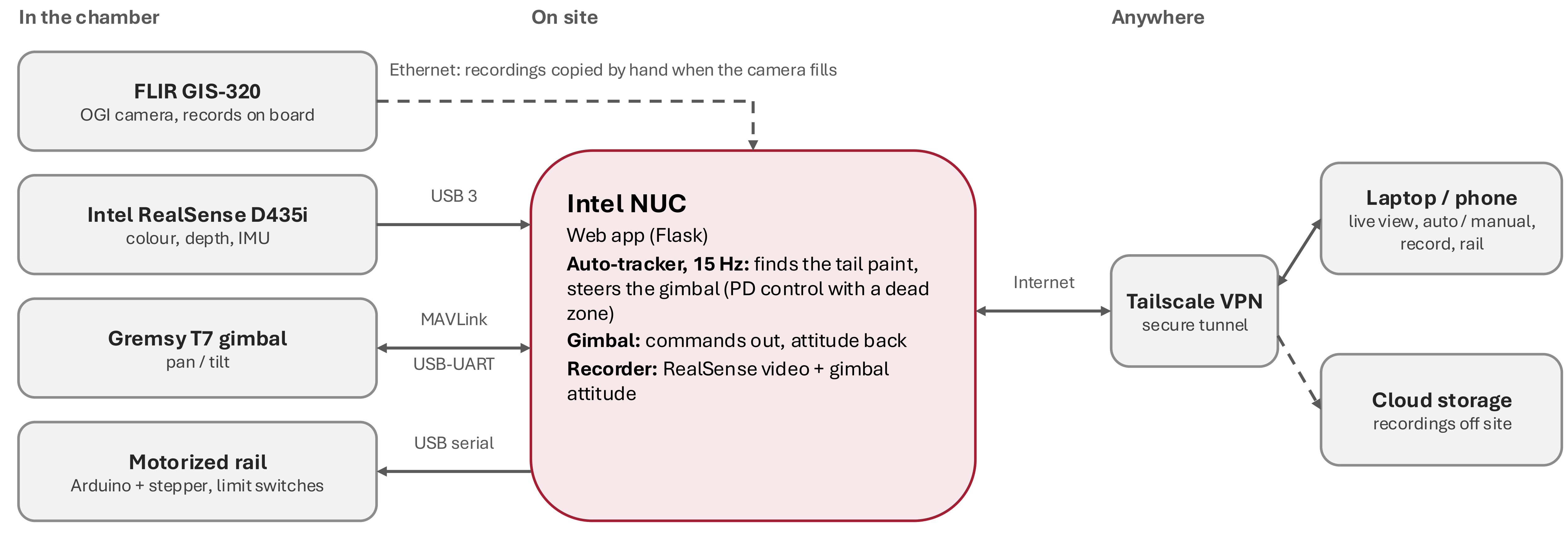
For the final four trial days, the payload rode a motorised ceiling rail (Arduino, stepper motor, and limit switches) between the two zones. Because the rail moves quietly and slowly, the cows tolerated it well—though curious animals occasionally came within 4 inches of the lens.
An onboard Intel NUC detects a stripe of livestock marking paint (tail paint) on the cow's nose bridge at 15 Hz and steers the gimbal via PD control with a dead zone, keeping the nostrils framed without chasing small twitches. Operators control live viewing, tracking, recording, and rail position day and night from a laptop or phone over a Tailscale VPN.
Hardware evolution across the chamber trials
05 · Automated stationary-scene curation
Screening recordings for stationary, in-profile scenes
Our spatiotemporal filter (§06) treats variations slower than ~0.5 s as background and faster fluctuations as candidate gas. That assumption holds only when the camera is stationary, the cow is in profile, and the black backdrop sits behind the nostrils.
Ideal geometry: stationary camera, cow in profile
Even in these well-framed clips, the warm head and reflective metal rails dominate the raw image while the breath plume remains invisible. Extracting that faint plume is the task of §06.
Excluded footage: motion and framing failures
06 · Revealing the plume
Selective filtering and windowed RMS activity
A breath plume changes the image by about a count; the camera's noise is 0.6 counts. Three steps separate the two: follow the slow background, average the noise away while letting fast changes through, and measure how much each pixel flickers.
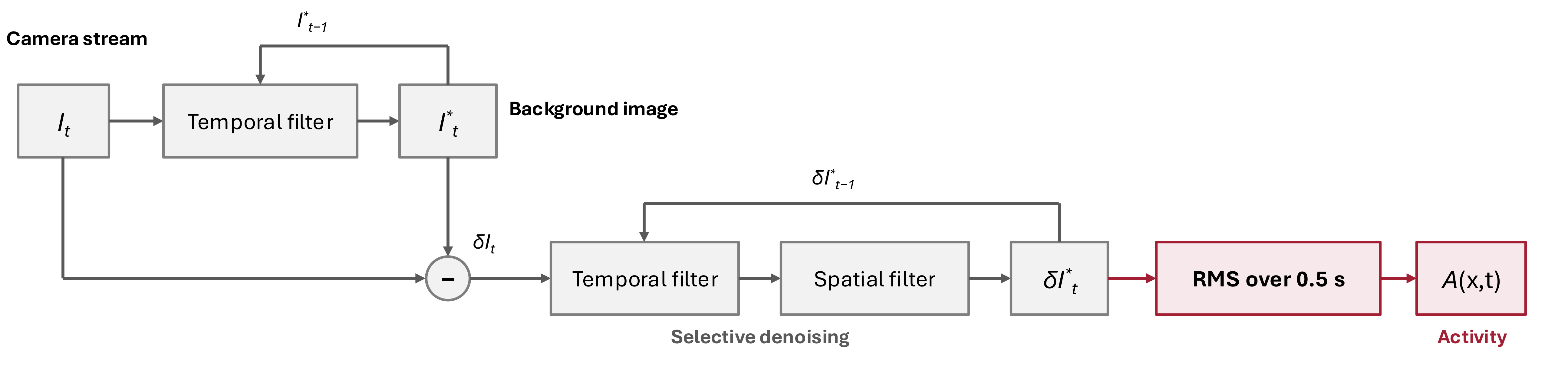
- 1Follow the background. An exponential temporal filter remembers about half a second (at 30 frames/s):\[ I^*_t = p_0\, I_t + (1 - p_0)\, I^*_{t-1}, \qquad p_0 = \tfrac{1}{15} \]
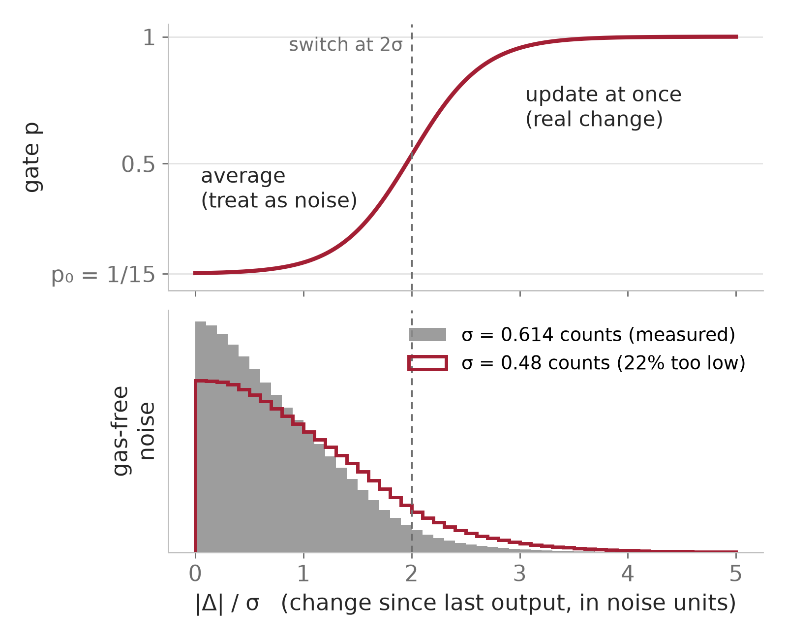
- 2Average noise, pass gas. The change from the background is filtered again, but its averaging switches off when a change is too big to be noise. A sigmoid gate in noise units sets the switch at 2σ:\[ \delta I^*_t = K * \Big[\, p\,(I_t - I^*_{t-1}) + (1-p)\,\delta I^*_{t-1} \Big], \qquad p = p_0 + \frac{1 - p_0}{1 + e^{-3(|\Delta|/\sigma - 2)}} \]where \(K\) is a 1-pixel spatial blur and \(\Delta\) is the step change from the previous filtered output.
- 3Measure the flicker. Turbulent eddies break a plume into puffs, so one pixel's column both shifts and flickers. The RMS over a 0.5 s window keeps both; camera noise averages to zero and adds only a fixed σ²:\[ A(x,t) = \sqrt{\operatorname{mean}_{0.5\,\text{s}}\big(\delta I^{*2}\big)}, \qquad A^2 = \underbrace{\big(\operatorname{mean}\,\delta I^*\big)^2}_{\text{shift}} + \underbrace{\operatorname{var}\,\delta I^*}_{\text{fluctuation}} \]
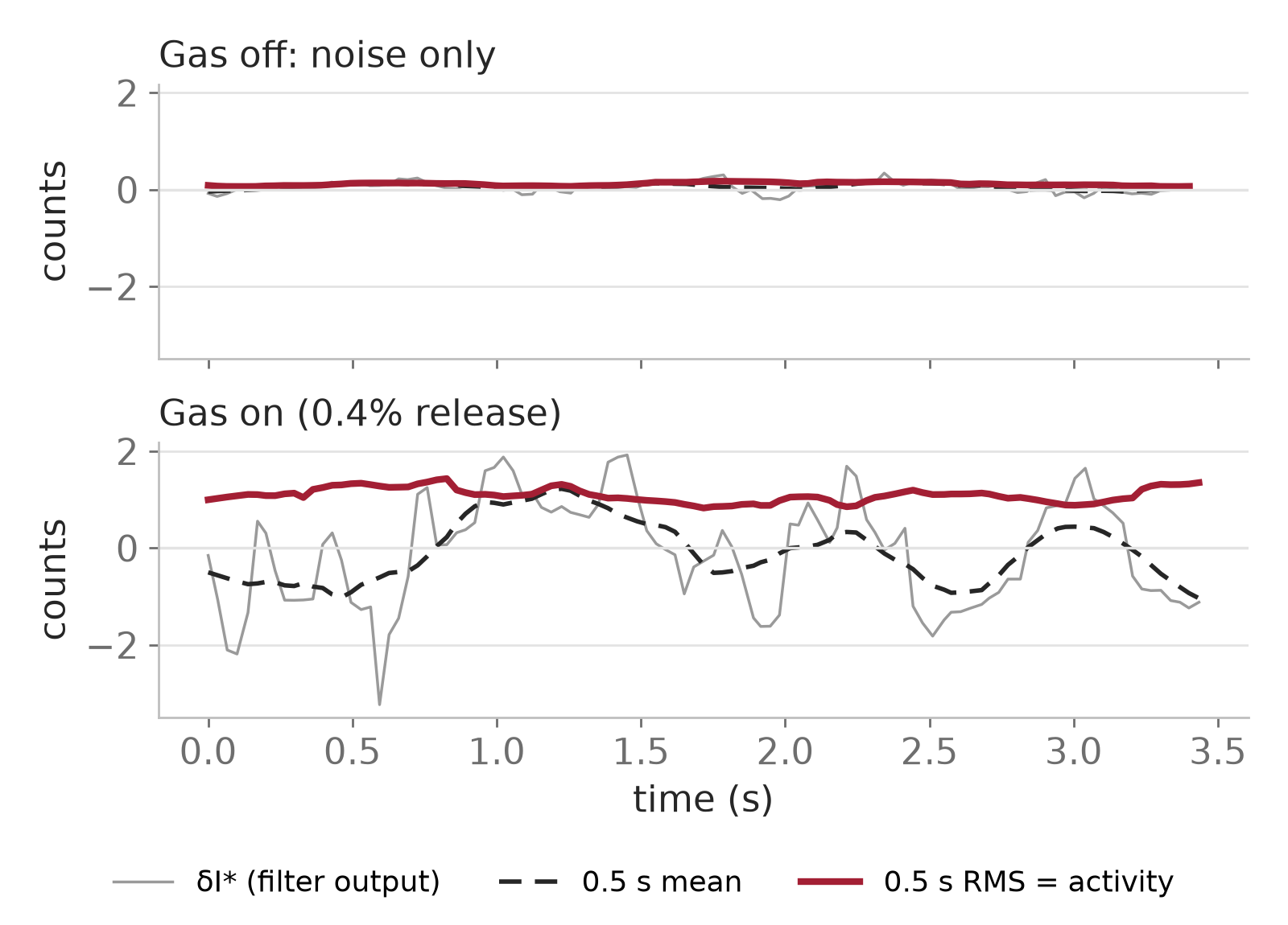
Controlled releases (0.4% methane): the windowed RMS detects 34% of gas pixels, against 15% from single frames at the same false-alarm rate (2.4×). 59% of the extra signal is in the fluctuation term. The full-trial analysis uses a 1 s window, which gives 3.4× (50% vs 15%) on the same release.
Measuring the noise: two σ, two jobs
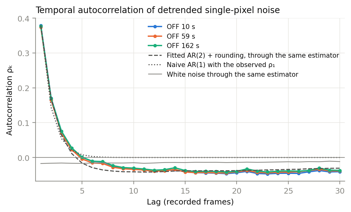
Every threshold in the pipeline is a multiple of a noise level, so we measured the noise instead of assuming it. Two levels matter: the raw pixel noise σgate, which places the filter's gate, and the much smaller noise of the filter's own output, σout, which sets the activity scale and the region thresholds of §08.
| σgate | σout | |
|---|---|---|
| What it is | Single-pixel noise of the raw counts | Gas-free level of the activity (windowed RMS) |
| Value | 0.614 counts (≈ 15 mK) | 0.12–0.18 counts on releases; 0.199 counts for cows (global), then per clip |
| Measured on | Three gas-free release clips, drift removed per pixel | Gas-free release clips; far background of every usable cow clip |
| Used for | The gate's switch at 2σgate | Activity units; region thresholds at 2σout and 3σout |
Details: the project's noise study (single-pixel temporal noise of the GIS-320 raw counts, October 2026) and the σout survey of the full run.
Tracing one clip through the filter stages
07 · Masking non-gas artifacts
Warm head motion and specular metal both mimic gas
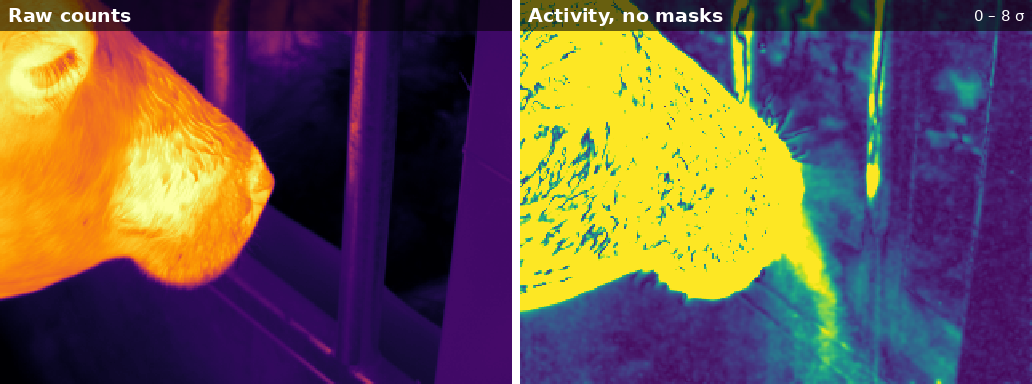

Masking in action
Some activity still leaks at the moving head's edge, just outside the 8 px margin. The pipeline now keeps a pixel masked for 15 frames (0.5 s) after the cow leaves it, because the background filter still remembers the warm head there.
08 · Segmenting candidate plume regions
3D hysteresis connected-component labeling in (x, y, t)
- 1Grow across voxels with activity ≥ 2σout (exceeded by ~1 in 1,000 gas-free samples).
- 2Seed at cores of ≥ 5 px with activity ≥ 3σout (~1 in 1,000,000 gas-free samples).
- 3Connect contiguous voxels in (x, y, t) so each evolving puff forms a single 3D volume.
- 4Keep regions with a seed that touch the outlet: a 10 px circle where the plume leaves the nose, clicked once per clip in review.
- 5Measure each candidate region's onset, duration, peak activity, area, and maximum reach from the outlet.
Two thresholds do what one can't. A high seed threshold means a region is almost never pure noise; a lower growing threshold lets each region spread to the plume's faint edges. Requiring the region to touch the nostril outlet rejects leftover clutter elsewhere in the frame.
09 · Next: cross-calibrating with the chamber
Fast optical plumes vs. the chamber's well-mixed response
The camera sees each burp as it happens. The chamber mixes all of them into its air, which is replaced over several minutes, so it sees a smoothed sum. Both should account for the same methane.
A burp of mass \(m\) raises a well-mixed chamber of volume \(V\) by \(m/V\) at once; the air flow \(Q\) then washes it out with time constant \(\tau = V/Q\). Flow times the area under the chamber's curve gives back the methane:
Here \(\Delta C\) is mass concentration above background—the analyzer's mole fraction in ppm multiplied by methane density (0.716 g/L at STP).
Our chamber. The Bioeconomy Science Institute chamber holds \(V\) = 15.8 m³ with an air flow of about 1.9 m³/min, so \(\tau = V/Q \approx\) 8.4 min. Fitting the decay after each door closure gives 9.5 min for CO₂ and 9.8 min for CH₄. A burp that lasts seconds is spread over about ten minutes in the chamber's record.
Multi-day chamber trial coverage
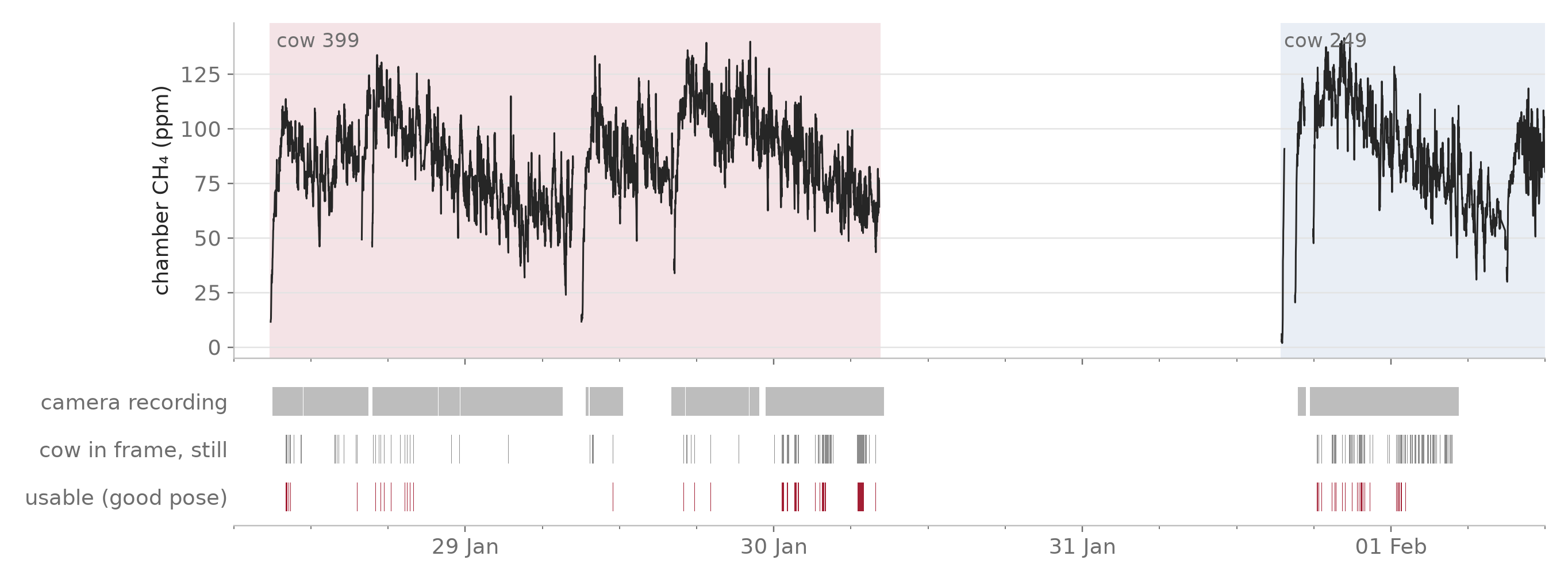
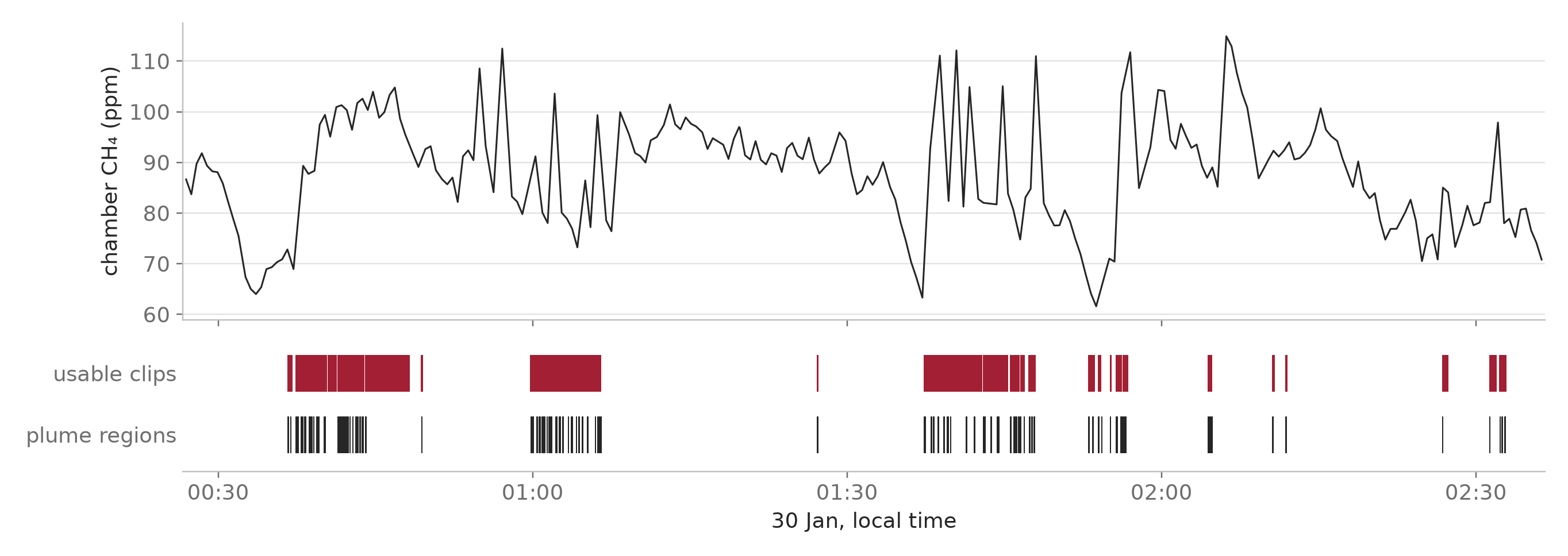
Next steps toward event-level quantification
- 1Synchronize clocks. Verify and lock the camera-to-analyzer time offset.
- 2Respect the chamber's lag. Its air takes about 9 minutes to turn over (measured 8.4–9.8 min), so compare totals over windows of at least one turnover, not single breaths.
- 3Rate vs production. Events per measured minute against the chamber's methane production (flow × CH₄ rise) in the same windows.
- 4Test temporal lead–lag. Check whether bursts of high-activity plume regions precede rises in the chamber analyzer trace.
- 5Behaviour, event by event. Because the camera sees single eructations as they happen, emissions can be lined up with what the cow is doing at that moment: eating, ruminating, lying down or standing, head position. Chamber and tracer methods average over minutes to days and cannot make that link. This is the next analysis, not yet a result.